

Transfer Function Estimation Matlab

Mathematical Models And Simulation Of Electrical Systems Mathematical Model System Differential Equations

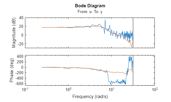
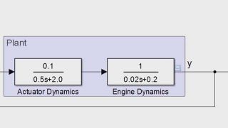
Estimate The Transfer Function Of An Unknown System Matlab Simulink

Estimating Transfer Functions And Process Models Video Matlab
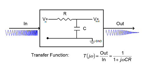
Estimate The Transfer Function Of A Circuit With Adalm1000 Matlab Simulink
Z8kmvelv Bffjm
Estimating Transfer Functions And Process Models Video Matlab

If one of the signals is a matrix and the other is a vector then the length of the vector must equal the number of rows in.
Transfer function estimation matlab. Signal processing functions estimate the transfer function based on measured data and compare the theoretical response of the circuit. After the estimation is completed we can compare the output of the model with the measured shaft angle. It can be any positive integer scalar and the default is 1.
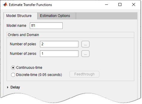
Use the tfest command specifying one pole no zeroes and an unknown inputoutput delay to estimate a transfer function. In the example below assume you are trying to find an estimate for the transfer function. Using functionality in toolboxes such as Data Acquisition Toolbox and Instrument Control Toolbox MATLAB can connect to configure and control hardware to make live measurements and use the measurements.
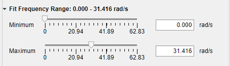
Load time-domain system response data z2 and use it to estimate a transfer function that contains two poles and one zero. For nonperiodic data the transfer function is estimated at 128 equally-spaced frequencies 1128128piTs. D iddata tdy tdu 1Fs.
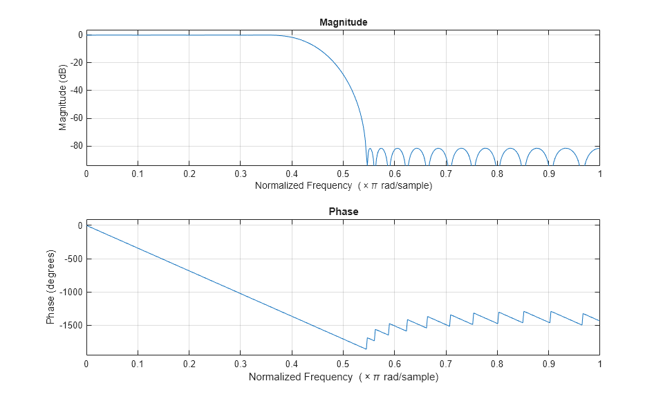
For that we use the new function tfest. This example shows how to use the Discrete Transfer Function Estimator block to estimate the magnitude and phase response of a continuous-time analog. Time domain data data.
The alias-free signal bandwidth BW the FFT length used in transfer estimation and the number of spectral averages used to smooth the estimate. Create Transfer Function Estimator. Data has 2 outputs 2 inputs and 1 408 samples.
From the physics of the problem we know that the heat exchanger can be described by a first order system with delay. 3162021 Estimates from Time Series Data. For nonperiodic data the transfer function is estimated at 128 equally-spaced frequencies 1128128piTs.
I2qkvcbhjyhnpm

On Off Control System Control System System Control

Estimating Transfer Functions And Process Models Video Matlab
Estimate Transfer Function Models In The System Identification App Matlab Simulink

Estimate The Transfer Function Of An Unknown System Matlab Simulink

Estimating Transfer Functions And Process Models Video Matlab

Optimum Wireless Power Transfer Using Lumped L Section Networks Networking Power Wireless
Estimate The Transfer Function Of An Unknown System Matlab Simulink

Matlab Central Steve On Image Processing Fourier Series Animation Using Phasor Addition Image Processing Space Science Mathematics
How To Use The Discrete Time Identified Transfer Function In Matlab

How To Use The Discrete Time Identified Transfer Function In Matlab

Plc Based Intelligent Traffic Control System Using Sensors Control System Sensor Programmable Logic Controllers

Genetic Algorithm Matlab Genetic Algorithm Information Visualization Algorithm
