Transfer Function Unit Step Response

The Unit Step Response
The Unit Step Response

Unit Step Response Of Three Processes With Transfer Functions Given In Download Scientific Diagram
Http Www Ee Ic Ac Uk Pcheung Teaching De2 Ee Lecture 207 20 20step 20response 20 20system 20behaviour 20 X1 Pdf
Http Www Ee Ic Ac Uk Pcheung Teaching De2 Ee Lecture 207 20 20step 20response 20 20system 20behaviour 20 X1 Pdf
The Unit Step Response
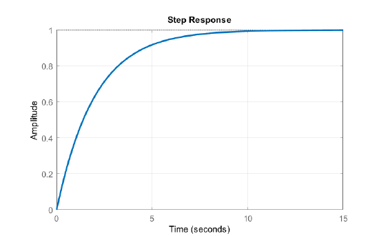
As shown a pole given by the transfer function Hs 1 s α has an inverse Laplace transform xt e αt for t 0.
Transfer function unit step response. We know the basic transfer function is given as. 0 1 x 0. Plotting step response.
3262020 Time Response of Second-Order system with Unit Step Input. S681818s s6 s10 The Laplace transform Es of the input signal unit step is Es frac1s The transfer function Gs relates the input and output by FsGs Es. The unit-step input is defined as.
A plot of the resulting step response is included at the end to validate the solution. Unit impulse response plots for some different cases This subsection contains some more plots that show the effect of pole locations and help illustrate the general trends. Function is known though the transfer function is more commonly used for the zero state response.
Let us first understand the time response of the undamped second-order system. This gives confidence in the calculation method for the transfer function. Using the closed-loop transfer function uδ u describe and assess the unit step response.
The step response of a system in a given initial state consists of the time evolution of its outputs when its control inputs are Heaviside step functions. Laplace transform of the unit step signal is We know the transfer function of the second order closed loop control system is. The impulse and step inputs are among prototype inputs used to characterize the response of the systems.
The Laplace transform Fs of the response of the system to a unit step input is Fs frac880. N 1 00381 From the results we got in previous slide the step response of the light bulb is a rising exponential with a time constant of t 0038. So the transfer function is determined by taking the Laplace transform with zero initial conditions and solving for V sF s To find the unit step response multiply the transfer function by the unit step 1s and solve by looking up the inverse transform in the Laplace Transform table Asymptotic exponential.

The Unit Step Response
Http Www Ee Ic Ac Uk Pcheung Teaching De2 Ee Lecture 207 20 20step 20response 20 20system 20behaviour 20 X1 Pdf
The Unit Step Response

Transient Response From Transfer Function Representation

Gate 2008 Ece Match Step Response Of Second Order System With Transfer Functions Youtube
The Unit Step Response

Nyquist Stability Criterion Examples And Matlab Coding Control Systems Engineering Coding Transfer Function

Finding Transfer Functions From Response Graphs Youtube

Gate 2006 Ece Transfer Function Of Unit Step Response Of A System Starting From Rest Ct Youtube
2 4 The Step Response Engineering Libretexts
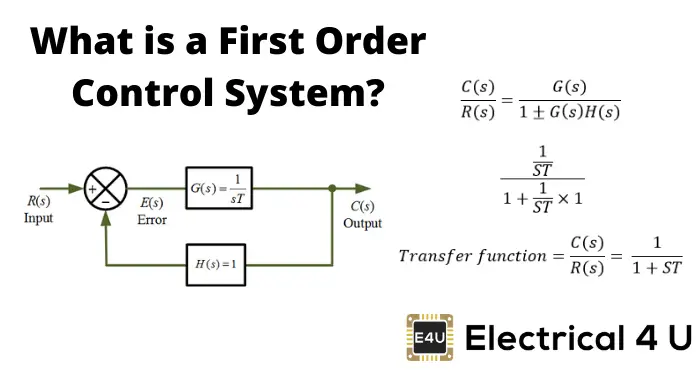
First Order Control System What Is It Rise Settling Time Formula Electrical4u

The Unit Step Response
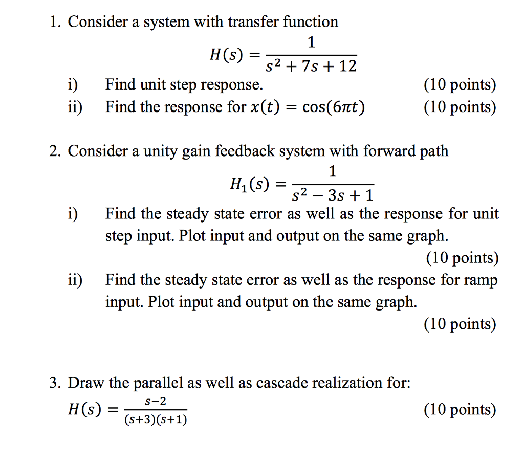
Solved Consider A System With Transfer Function H S 1 Chegg Com